Loading Geospatial Data in RStudio
Last updated: 2024-12-27
Checks: 7 0
Knit directory: R_tutorial/
This reproducible R Markdown analysis was created with workflowr (version 1.7.1). The Checks tab describes the reproducibility checks that were applied when the results were created. The Past versions tab lists the development history.
Great! Since the R Markdown file has been committed to the Git repository, you know the exact version of the code that produced these results.
Great job! The global environment was empty. Objects defined in the global environment can affect the analysis in your R Markdown file in unknown ways. For reproduciblity it’s best to always run the code in an empty environment.
The command set.seed(20241223) was run prior to running
the code in the R Markdown file. Setting a seed ensures that any results
that rely on randomness, e.g. subsampling or permutations, are
reproducible.
Great job! Recording the operating system, R version, and package versions is critical for reproducibility.
Nice! There were no cached chunks for this analysis, so you can be confident that you successfully produced the results during this run.
Great job! Using relative paths to the files within your workflowr project makes it easier to run your code on other machines.
Great! You are using Git for version control. Tracking code development and connecting the code version to the results is critical for reproducibility.
The results in this page were generated with repository version 8269de6. See the Past versions tab to see a history of the changes made to the R Markdown and HTML files.
Note that you need to be careful to ensure that all relevant files for
the analysis have been committed to Git prior to generating the results
(you can use wflow_publish or
wflow_git_commit). workflowr only checks the R Markdown
file, but you know if there are other scripts or data files that it
depends on. Below is the status of the Git repository when the results
were generated:
Ignored files:
    Ignored:    .Rhistory
    Ignored:    .Rproj.user/

Untracked files:
    Untracked:  analysis/Basic_Operations_with_Raster_Data.Rmd
    Untracked:  analysis/Resources.Rmd

Unstaged changes:
    Modified:   analysis/Understanding_Geospatial_Data.Rmd
    Modified:   analysis/_site.yml
    Deleted:    analysis/about.Rmd
Note that any generated files, e.g. HTML, png, CSS, etc., are not included in this status report because it is ok for generated content to have uncommitted changes.
These are the previous versions of the repository in which changes were
made to the R Markdown
(analysis/Loading_Geospatial_Data_in_RStudio.Rmd) and HTML
(docs/Loading_Geospatial_Data_in_RStudio.html) files. If
you’ve configured a remote Git repository (see
?wflow_git_remote), click on the hyperlinks in the table
below to view the files as they were in that past version.
| File | Version | Author | Date | Message |
|---|---|---|---|---|
| Rmd | 8269de6 | Ohm-Np | 2024-12-27 | wflow_publish("analysis/Loading_Geospatial_Data_in_RStudio.Rmd") |
| html | 504b7c8 | Ohm-Np | 2024-12-25 | Build site. |
| Rmd | d205c20 | Ohm-Np | 2024-12-25 | wflow_publish("analysis/Loading_Geospatial_Data_in_RStudio.Rmd") |
| html | c25291f | Ohm-Np | 2024-12-25 | Build site. |
| Rmd | 69eb640 | Ohm-Np | 2024-12-25 | wflow_publish("analysis/Loading_Geospatial_Data_in_RStudio.Rmd") |
| html | c7cee43 | Ohm-Np | 2024-12-25 | Build site. |
| Rmd | 2c2603b | Ohm-Np | 2024-12-25 | wflow_publish("analysis/Loading_Geospatial_Data_in_RStudio.Rmd") |
Once you have RStudio set up and the required packages installed, the next step is to load your geospatial data into R. R provides several powerful packages for importing, manipulating, and analyzing spatial data. Two of the most commonly used packages for handling vector and raster data are sf and terra, respectively. These packages make it easy to work with geospatial data within RStudio, allowing you to perform spatial analysis, visualization, and data manipulation seamlessly.
Importing Vector Data
The sf (Simple Features) package is the go-to tool for working with vector data in R. It supports various vector file formats such as Shapefile (.shp), GeoJSON, and GeoPackage (.gpkg). One of the advantages of using sf is that it provides a simple and consistent interface for working with vector data, making it easy to import, manipulate, and analyze geospatial features. Additionally, sf integrates well with the tidyverse ecosystem, allowing for smooth workflows in data manipulation and visualization.
To load vector data using the sf package, you typically use either st_read() or read_sf() function.
In this tutorial, I am using a .gpkg file which is made available on GitHub. You can download it by clicking this link.
# Load the sf package
library(sf)

# Import your downloaded gpkg file
# don't forget to provide the path where you have downloaded it locally
vector_data <- read_sf("data/vector/kanchanpur.gpkg")

# View the first few rows of the data
head(vector_data)
Simple feature collection with 6 features and 1 field
Geometry type: MULTIPOLYGON
Dimension: XY
Bounding box: xmin: 80.06014 ymin: 28.64567 xmax: 80.55588 ymax: 29.05851
Geodetic CRS: WGS 84
# A tibble: 6 × 2
NAME geom
<chr> <MULTIPOLYGON [°]>
1 BaisiBichawa (((80.49934 28.64667, 80.49709 28.64866, 80.49709 28.65089, 80.4…
2 Beldandi (((80.25229 28.75782, 80.25377 28.7646, 80.25588 28.76808, 80.25…
3 Chandani (((80.10973 28.98432, 80.10986 28.97376, 80.10738 28.96319, 80.1…
4 Daijee (((80.34424 29.05416, 80.34449 29.04956, 80.34698 29.04397, 80.3…
5 Dekhatbhuli (((80.44701 28.78921, 80.43608 28.78623, 80.4316 28.78623, 80.42…
6 Dodhara (((80.10042 28.88838, 80.09917 28.87645, 80.10327 28.87297, 80.1…# Lets plot the data to see how it looks
plot(vector_data, main = "Kanchanpur district (Nepal)")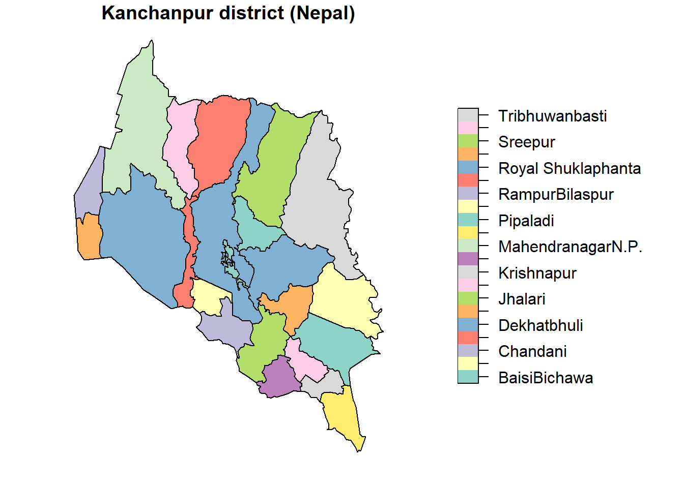
| Version | Author | Date |
|---|---|---|
| c7cee43 | Ohm-Np | 2024-12-25 |
In this example, read_sf() reads the GeoPackage and loads into an sf object. The sf object contains both the geometric data (polygons in this case) and the any associated attribute data (names of VDCs, Municipalities). As you can see from the data and plot above, this gpkg file is of Kanchanpur dictrict from Nepal. Once the data is loaded, you can perform a wide range of operations, such as subsetting, transforming projections, and performing spatial queries.
Importing Raster Data
The terra package is specifically designed for raster data and provides improved performance and easier handling of large datasets compared to the raster package. The terra package supports a wide variety of raster formats, including GeoTIFF (.tif), ASCII, and more.
To load raster data using terra, you use the rast() function. In this tutorial, I am using .tif files which are available on GitHub. You can download it by clicking here: Land Cover 2015 & Land Cover 2019.
# Load the terra package
library(terra)

# Import your downloaded tif file
# don't forget to provide the path where you have downloaded it locally
raster_data <- rast("data/raster/landcover_2015.tif")

# View basic information about the raster
raster_data
class : SpatRaster
dimensions : 590, 505, 1 (nrow, ncol, nlyr)
resolution : 0.0009920635, 0.0009920635 (x, y)
extent : 80.06052, 80.56151, 28.55159, 29.1369 (xmin, xmax, ymin, ymax)
coord. ref. : lon/lat WGS 84
source : landcover_2015.tif
name : E080N40_PROBAV_LC100_global_v3~e-Classification-map_EPSG-4326
min value : 20
max value : 126
unit : None # Lets plot the data to see how it looks
plot(raster_data)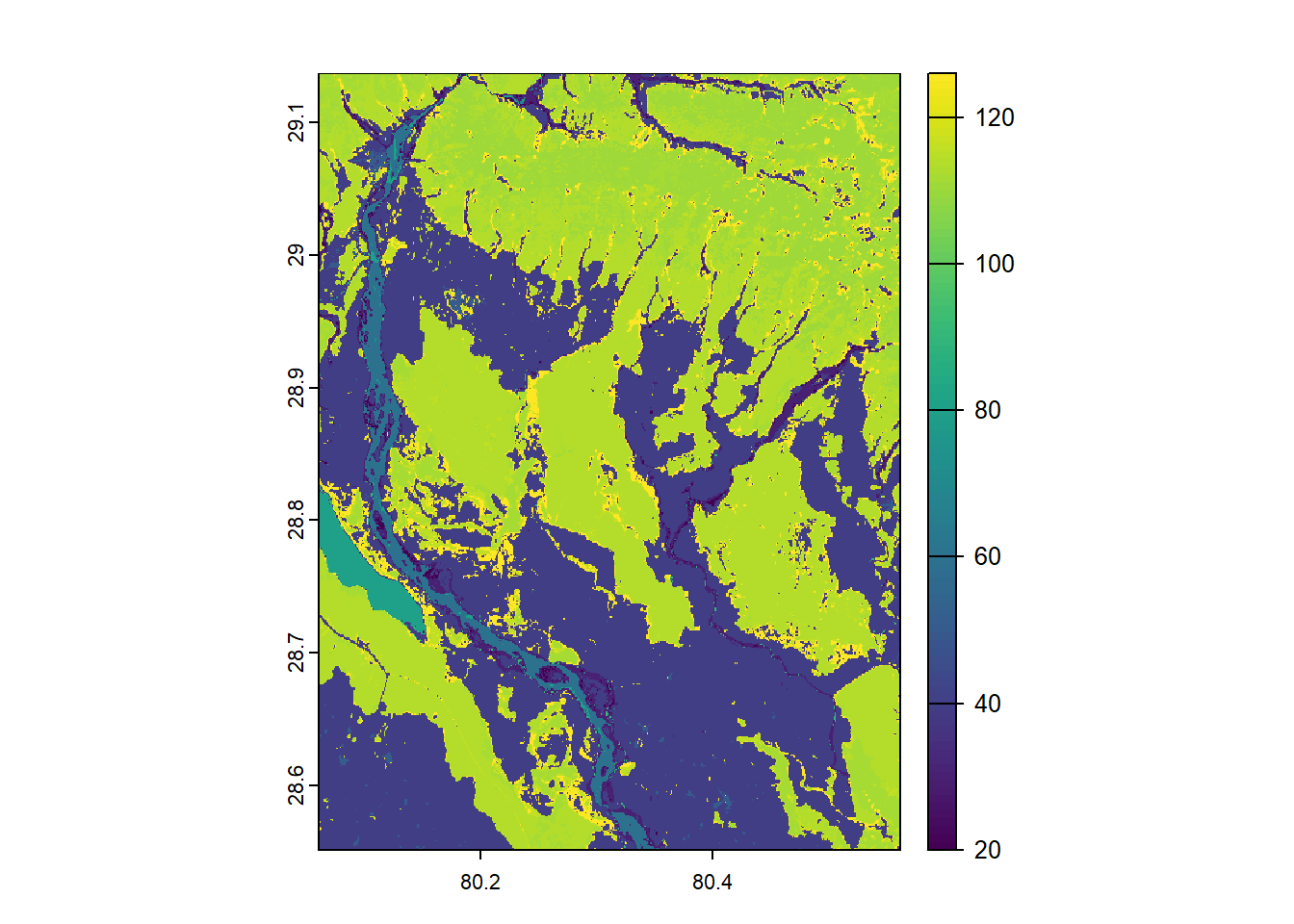
| Version | Author | Date |
|---|---|---|
| c7cee43 | Ohm-Np | 2024-12-25 |
In this example, rast() loads a raster file into a SpatRaster object. This object contains both the spatial grid (array of pixels) and the values for each pixel. The terra package makes it easier to manipulate raster data, offering functions to crop, mask, reclassify, and perform raster algebra operations.
Now that we are familiar with R, RStudio, the essential R packages for geospatial analysis, and the process of importing vector and raster data, it’s time to dive deeper into basic geospatial operations.
sessionInfo()R version 4.4.0 (2024-04-24 ucrt)
Platform: x86_64-w64-mingw32/x64
Running under: Windows 11 x64 (build 22631)
Matrix products: default
locale:
[1] LC_COLLATE=English_Germany.utf8 LC_CTYPE=English_Germany.utf8
[3] LC_MONETARY=English_Germany.utf8 LC_NUMERIC=C
[5] LC_TIME=English_Germany.utf8
time zone: Europe/Berlin
tzcode source: internal
attached base packages:
[1] stats graphics grDevices utils datasets methods base
other attached packages:
[1] terra_1.8-5 sf_1.0-19 workflowr_1.7.1
loaded via a namespace (and not attached):
[1] jsonlite_1.8.8 highr_0.11 compiler_4.4.0 promises_1.3.0
[5] Rcpp_1.0.13 stringr_1.5.1 git2r_0.33.0 callr_3.7.6
[9] later_1.3.2 jquerylib_0.1.4 yaml_2.3.10 fastmap_1.2.0
[13] R6_2.5.1 classInt_0.4-10 knitr_1.48 tibble_3.2.1
[17] units_0.8-5 rprojroot_2.0.4 DBI_1.2.3 bslib_0.8.0
[21] pillar_1.9.0 rlang_1.1.4 utf8_1.2.4 cachem_1.1.0
[25] stringi_1.8.4 httpuv_1.6.15 xfun_0.47 getPass_0.2-4
[29] fs_1.6.4 sass_0.4.9 cli_3.6.3 magrittr_2.0.3
[33] class_7.3-22 ps_1.8.1 grid_4.4.0 digest_0.6.36
[37] processx_3.8.4 rstudioapi_0.16.0 lifecycle_1.0.4 vctrs_0.6.5
[41] KernSmooth_2.23-22 proxy_0.4-27 evaluate_0.24.0 glue_1.7.0
[45] whisker_0.4.1 codetools_0.2-20 e1071_1.7-16 fansi_1.0.6
[49] rmarkdown_2.28 httr_1.4.7 tools_4.4.0 pkgconfig_2.0.3
[53] htmltools_0.5.8.1